Application to high resolution spatial transcriptomics data

This tutorial demonstrates how to apply SpaCET to a colorectal cancer Slide-seq dataset from Zhao et al, 2021. Each bead is 10 µm in diameter covering 1-2 cells. Before running the tutorial, make sure that the SpaCET package and its dependencies have been installed.

Create SpaCET object

User need create.SpaCET.object to create a SpaCET object by preparing four types of input data referring to a tumor ST sample.

1. spatial transcriptomics count data. The spatial transcriptomics count data must be in the format of matrix with gene name (row) x spot ID (column).
2. spatial location information. The spot coordinates should be in the format of matrix with spot ID (row) x coordinates (column). This 1st and 2nd columns represent X and Y coordinates, respectively.
3. path to the H&E image file. The image path can be NA if unavailable.
4. platform.

library(SpaCET)

hiresST_Path <- system.file("extdata", 'hiresST_CRC', package = 'SpaCET')

# load count matrix
load(paste0(hiresST_Path,"/counts.rda"))

# show count matrix
counts[1:6,1:5]

## 6 x 5 sparse Matrix of class "dgCMatrix"
##         b1 b2 b3 b4 b5
## A1BG     .  .  .  .  .
## A1CF     .  1  2  1  1
## A2M      .  .  .  .  .
## A2ML1    .  .  .  .  .
## A3GALT2  .  .  .  .  .
## A4GALT   .  .  .  .  .

# load count matrix
load(paste0(hiresST_Path,"/spotCoordinates.rda"))

# show count matrix
head(spotCoordinates)

##    coordinate_x_um coordinate_y_um
## b1        2364.115        3072.225
## b2        3484.520        1734.005
## b3        2279.745        2951.975
## b4        3061.825        1556.490
## b5        2274.220        2982.525
## b6        2986.945        1603.680

# create a SpaCET object.
SpaCET_obj <- create.SpaCET.object(
  counts=counts,
  spotCoordinates=spotCoordinates,
  metaData=NULL,
  imagePath=NA,
  platform = "SlideSeq"
)

# show this object.
str(SpaCET_obj)

Deconvolve ST data

We use the in-house reference to deconvolve this ST sample.

# deconvolve ST data; ~30 minutes
SpaCET_obj <- SpaCET.deconvolution(SpaCET_obj, cancerType="CRC", coreNo=6)
# Since Windows does not support parallel computation, please set coreNo=1 for Windows OS.

# show the ST deconvolution results
SpaCET_obj@results$deconvolution$propMat[1:13,1:3]

##             b1 b2 b3
## Malignant    1  1  1
## CAF          0  0  0
## Endothelial  0  0  0
## Plasma       0  0  0
## B cell       0  0  0
## T CD4        0  0  0
## T CD8        0  0  0
## NK           0  0  0
## cDC          0  0  0
## pDC          0  0  0
## Macrophage   0  0  0
## Mast         0  0  0
## Neutrophil   0  0  0
``

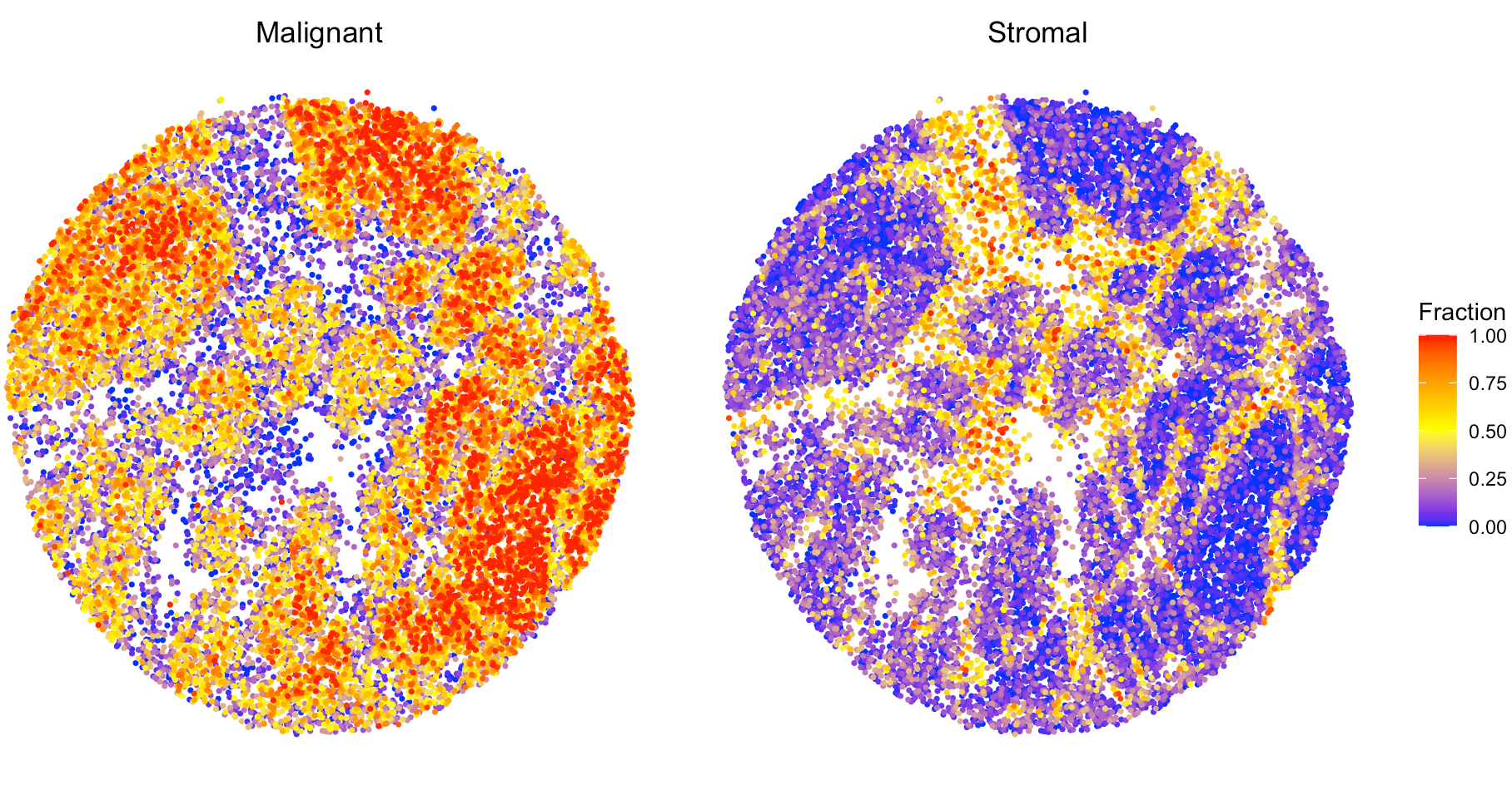
## Visualize the cell type proportion

We provide `SpaCET.visualize.spatialFeature` to present the spatial distribution of cell types. `spatialFeatures` could be a vector of cell types. If user would like to visualize multiple cell types in a single panel, you can assign a list to `spatialFeatures`. For example, combine CAF and endothelial cell types into stromal cell.

``` r
# show the spatial distribution of malignant cells and macrophages.
SpaCET.visualize.spatialFeature(
  SpaCET_obj, 
  spatialType = "CellFraction", 
  spatialFeatures = list(Malignant=c("Malignant"),Stromal=c("CAF","Endothelial")),
  sameScaleForFraction = TRUE,
  pointSize = 0.6
)

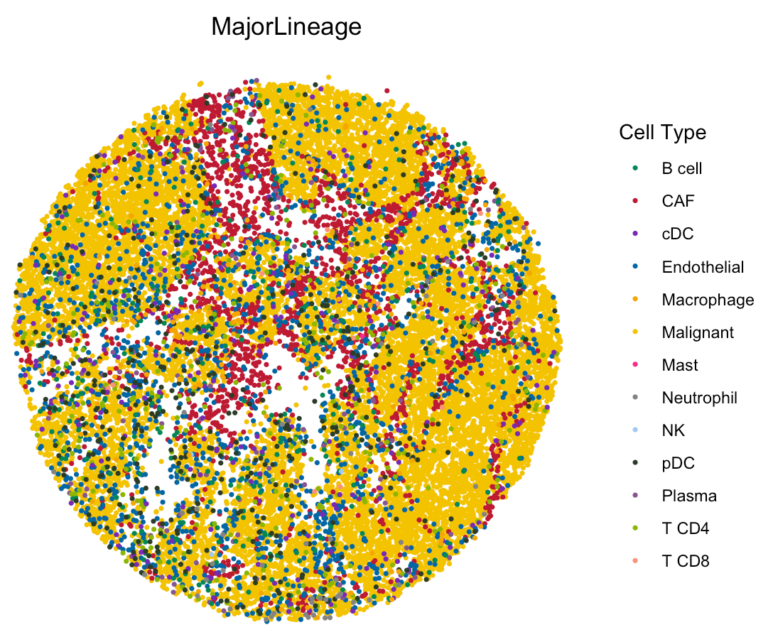
User can check the most abundant cell type in each bead by setting spatialType as “MostAbundantCellType”. spatialFeatures could be “MajorLineage” or “SubLineage”.

# load the color for cell types
load(paste0(hiresST_Path,"/colors_vector.rda"))

# show colors
head(colors_vector,3)

## Malignant            CAF    Endothelial
## "#f3c300"      "#be0032"      "#0067a5"

# show the spatial distribution of all cell types.
SpaCET.visualize.spatialFeature(
  SpaCET_obj, 
  spatialType = "MostAbundantCellType", 
  spatialFeatures = "MajorLineage", 
  colors = colors_vector,
  pointSize = 0.6
)